Load OMF Project

Load and visualize an OMF project file

Originally from: https://opengeovis.github.io/omfvista/examples/load-project.html

# sphinx_gallery_thumbnail_number = 3
import omfvista
import pooch
import pyvista as pv

Load the project into an pyvista.MultiBlock dataset

url = "https://raw.githubusercontent.com/pyvista/vtk-data/master/Data/test_file.omf"
file_path = pooch.retrieve(url=url, known_hash=None)

project = omfvista.load_project(file_path)
print(project)

MultiBlock (0x7f2f38ffa040)
  N Blocks    9
  X Bounds    443941.105, 447059.611
  Y Bounds    491941.536, 495059.859
  Z Bounds    2330.000, 3555.942

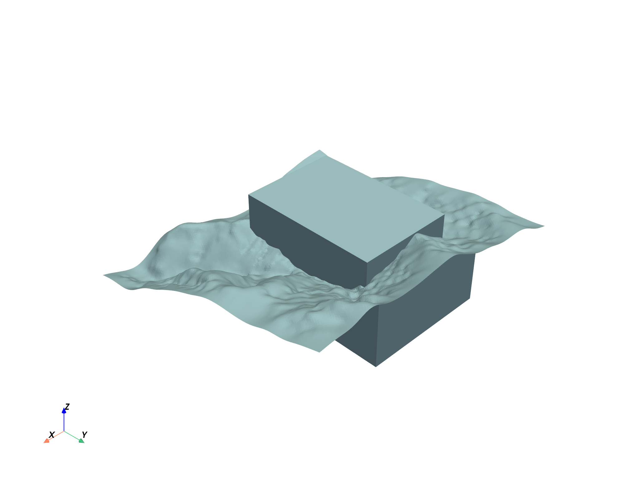
Once the data is loaded as a pyvista.MultiBlock dataset from omfvista, then that object can be directly used for interactive 3D visualization from pyvista:

project.plot()

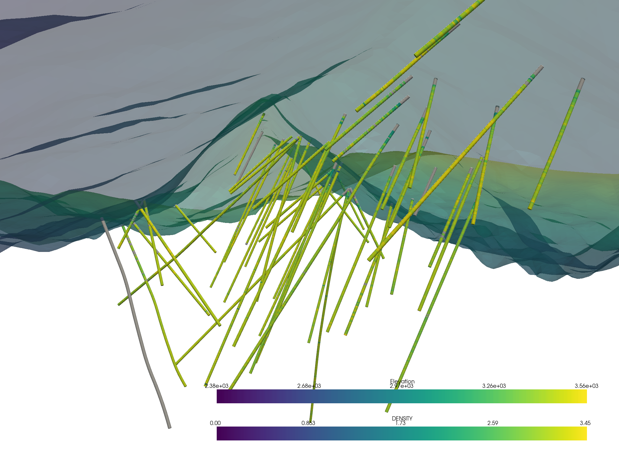
Or an interactive scene can be created and manipulated to create a compelling figure directly in a Jupyter notebook. First, grab the elements from the project:

# Grab a few elements of interest and plot em up!
vol = project["Block Model"]
assay = project["wolfpass_WP_assay"]
topo = project["Topography"]
dacite = project["Dacite"]

assay.set_active_scalars("DENSITY")

p = pv.Plotter()
p.add_mesh(assay.tube(radius=3))
p.add_mesh(topo, opacity=0.5)
p.camera_position = [
    (445542.1943310096, 491993.83439313783, 2319.4833541935445),
    (445279.0538059701, 493496.6896061105, 2751.562316285356),
    (-0.03677380086746433, -0.2820672798388477, 0.9586895937758338),
]
p.show()

Then apply a filtering tool from pyvista to the volumetric data:

# Threshold the volumetric data
thresh_vol = vol.threshold([1.09, 4.20])
print(thresh_vol)

UnstructuredGrid (0x7f2f39bfa040)
  N Cells:    92525
  N Points:   107807
  X Bounds:   4.447e+05, 4.457e+05
  Y Bounds:   4.929e+05, 4.942e+05
  Z Bounds:   2.330e+03, 3.110e+03
  N Arrays:   1

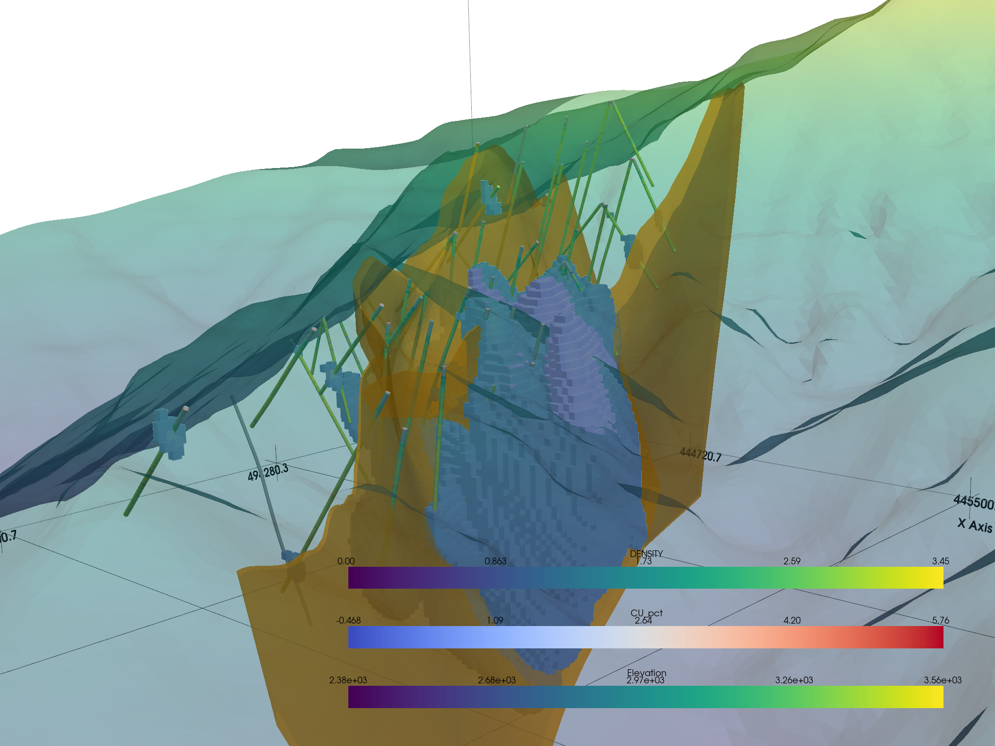
Then you can put it all in one environment!

# Create a plotting window
p = pv.Plotter()
# Add the bounds axis
p.show_grid()
p.add_bounding_box()

# Add our datasets
p.add_mesh(topo, opacity=0.5)
p.add_mesh(
    dacite,
    color="orange",
    opacity=0.6,
)
p.add_mesh(thresh_vol, cmap="coolwarm", clim=vol.get_data_range())

# Add the assay logs: use a tube filter that various the radius by an attribute
p.add_mesh(assay.tube(radius=3), cmap="viridis")
p.camera_position = [
    (446842.54037898243, 492089.0563631193, 3229.5037597889404),
    (445265.2503466077, 493747.3230470255, 2799.8853219866005),
    (-0.10728419235836695, 0.1524885965210015, 0.9824649255831316),
]
p.show()