Note
Go to the end to download the full example code
Kriging with GSTools
This example utilizes data available from the FORGE geothermal reserach site’s 2019 Geothermal Design Challenge. In this example, the data is archived in the Open Mining Format v1 (OMF) specification and the omfvista software is leverage to load those data into a PyVista MultiBlock data structure.
The goal of this workflow is to create a 3D temperature model by kriging the Observed Temperature data (sparse observational data). The open-source, Python software GSTools is used to perform variogram analysis and kriging of the temperature data onto a PyVista mesh to create the 3D model.
import PVGeo

# sphinx_gallery_thumbnail_number = 4
from gstools import Exponential, krige, vario_estimate_unstructured
from gstools.covmodel.plot import plot_variogram
import matplotlib.pyplot as plt
import numpy as np
import omfvista
import pooch
import pyvista as pv
Load the Data
For this project, we have two data archives in the Open Mining Format (OMF) specification and we will use one of PyVista’s companion projects, omfvista to load those data archives into PyVista a MultiBlock dataset.
url = "https://dl.dropbox.com/s/3cuxvurj8zubchb/FORGE.omf?dl=0"
path = pooch.retrieve(url=url, known_hash=None)

project = omfvista.load_project(path)
project
Initial Inspection
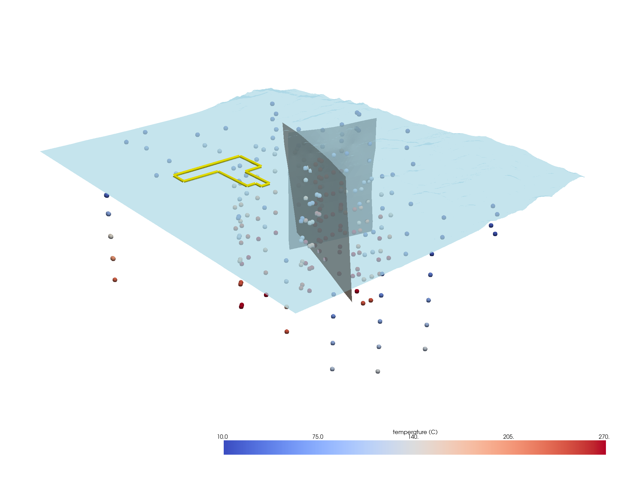
Now we can go ahead and create an integrated visualization of all of the data available to us.
p = pv.Plotter(window_size=np.array([1024, 768]) * 2)
p.add_mesh(project["Site Boundary"], color="yellow", render_lines_as_tubes=True, line_width=10)
p.add_mesh(project["Terrain"], opacity=0.7, lighting=False)
p.add_mesh(project["Opal Mound Fault"], color="brown", opacity=0.7)
p.add_mesh(project["Negro Mag Fault"], color="lightblue", opacity=0.7)
p.add_mesh(
    project["Observed Temperature"],
    cmap="coolwarm",
    clim=[10, 270],
    point_size=15,
    render_points_as_spheres=True,
)

p.camera_position = [
    (315661.9406719345, 4234675.528454831, 15167.291249498076),
    (337498.00521202036, 4260818.504034578, -1261.5688408692681),
    (0.2708862567924439, 0.3397398234107863, 0.9006650255615491),
]
p.show()
Kriging
Now we will use an external library, [gstools](https://geostat-framework.github.io), to krige the temperature probe data into a 3D temperature model of the subsurface.
Choosing a Model Space
We start out by creating the 3D model space as a PyVista UniformGrid that encompasses the project region. The following were chosen manually:
# Create the kriging grid
grid = pv.UniformGrid()
# Bottom south-west corner
grid.origin = (329700, 4252600, -2700)
# Cell sizes
grid.spacing = (250, 250, 50)
# Number of cells in each direction
grid.dimensions = (60, 75, 100)
/opt/hostedtoolcache/Python/3.8.18/x64/lib/python3.8/site-packages/pyvista/core/grid.py:912: PyVistaDeprecationWarning: `UniformGrid` is deprecated. Use `ImageData` instead.
  warnings.warn(
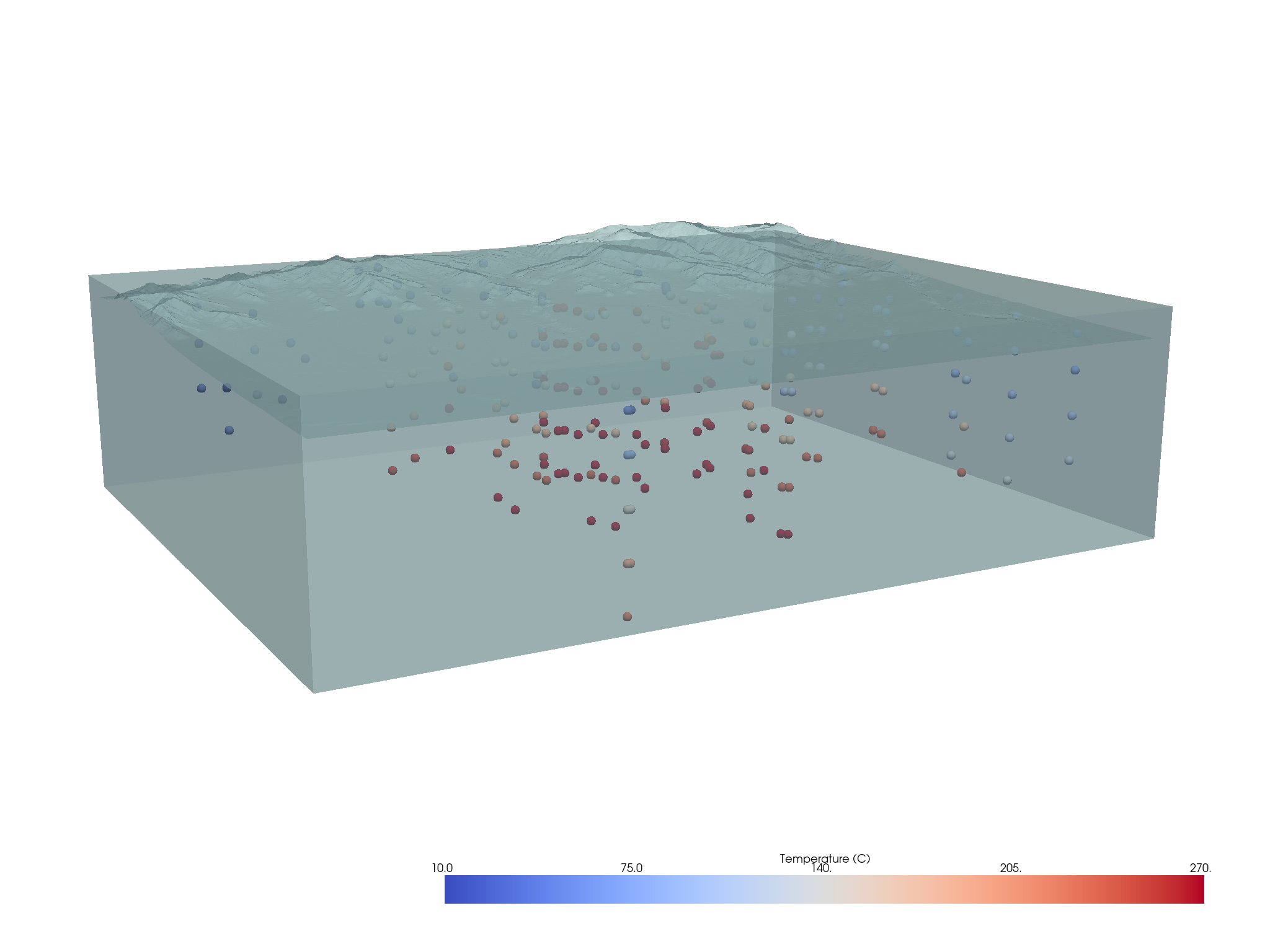
Visually inspect the kriging grid in relation to data
p = pv.Plotter(window_size=np.array([1024, 768]) * 2)
p.add_mesh(grid, opacity=0.5, color=True)
p.add_mesh(project["Terrain"], opacity=0.75)
p.add_mesh(
    project["Observed Temperature"],
    cmap="coolwarm",
    point_size=15,
    render_points_as_spheres=True,
    scalar_bar_args={"title": "Temperature (C)"},
)
p.camera_position = [
    (303509.4197523619, 4279629.689766085, 8053.049483835099),
    (336316.405356571, 4261479.748583805, -1756.358124546427),
    (0.22299463811939535, -0.11978828465250713, 0.9674317331109259),
]
p.show()
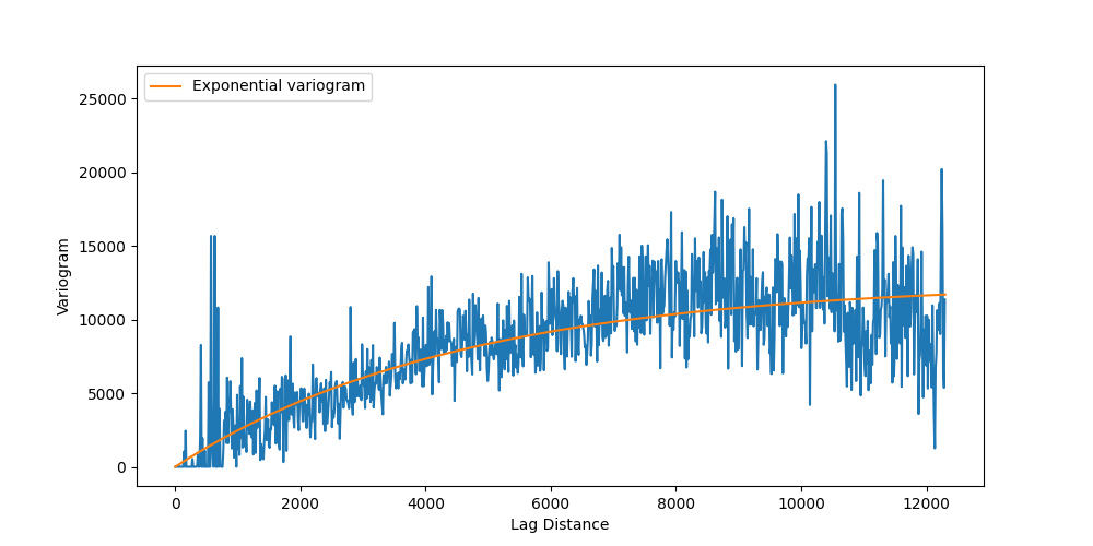
Variogram Analysis
Next, we need to compute a variogram for the temperature probe data and fit that variogram to an exponential model
bins = np.linspace(0, 12300, 1000)
bin_center, gamma = vario_estimate_unstructured(
    project["Observed Temperature"].points.T,
    project["Observed Temperature"]["temperature (C)"],
    bins,
)


fit_model = Exponential(dim=3)
fit_model.fit_variogram(bin_center, gamma, nugget=False)

plt.figure(figsize=(10, 5))
plt.plot(bin_center, gamma)
plot_variogram(fit_model, x_max=bins[-1], ax=plt.gca())
plt.xlabel("Lag Distance")
plt.ylabel("Variogram")
plt.show()
Performing the Kriging
Then we pass the fitted exponential model when instantiating the kriging operator from GSTools.
# Create the kriging model
krig = krige.Ordinary(
    fit_model,
    project["Observed Temperature"].points.T,
    project["Observed Temperature"]["temperature (C)"],
)
After instantiating the kriging operator, we can have it operate on the nodes of our 3D grid that we created earlier and collect the results back onto the grid.
krig.mesh(
    grid,
    name="temperature (C)",
)
(array([116.47283434, 117.61429646, 118.68575325, ...,  38.14187354,
        39.55052588,  40.95368015]), array([8097.97806581, 7671.55310286, 7233.87779749, ..., 8755.22696965,
       9108.52838828, 9445.1394835 ]))
And now the grid model has the temperature scalar field and kriging variance as data arrays.
project["Kriged Temperature Model"] = grid
project
Post-Processing
We can use a filter from PVGeo to extract the region of the temperature model that is beneath the topography surface as the kriging did not account for the surface boundary.
# Instantiate the algorithm
extractor = PVGeo.grids.ExtractTopography(tolerance=10, remove=True)
# Apply the algorithm to the PyVista grid using the topography surface
subsurface = extractor.apply(grid, project["Terrain"])
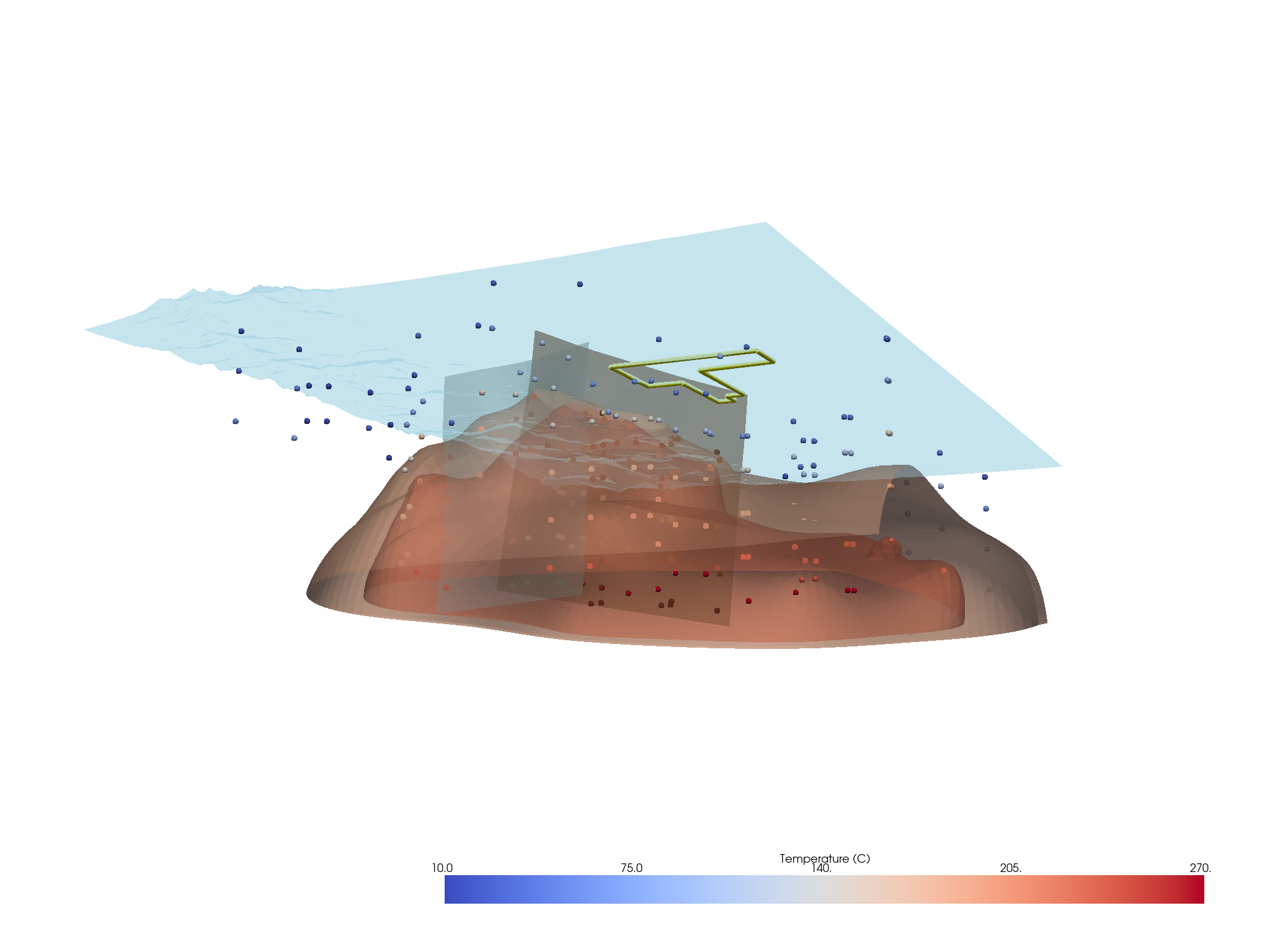
Resulting Visualization
# Create the main figure
def add_contents(p):
    """A helper to add data to scenes."""
    p.add_mesh(
        project["Site Boundary"].tube(50),
        color="yellow",
    )
    p.add_mesh(project["Terrain"], opacity=0.7, lighting=False)

    p.add_mesh(project["Opal Mound Fault"], color="brown", opacity=0.75)
    p.add_mesh(project["Negro Mag Fault"], color="lightblue", opacity=0.75)

    p.add_mesh(
        subsurface.ctp().contour([175, 225], scalars="temperature (C)"),
        name="the model",
        scalars="temperature (C)",
        cmap="coolwarm",
        clim=[10, 270],
        opacity=0.9,
        scalar_bar_args={"title": "Temperature (C)"},
    )
    p.add_mesh(
        project["Observed Temperature"],
        cmap="coolwarm",
        clim=[10, 270],
        render_points_as_spheres=True,
        point_size=10,
        scalar_bar_args={"title": "Temperature (C)"},
    )

    return


p = pv.Plotter()

add_contents(p)

p.camera_position = [
    (319663.46494887985, 4294870.4704494225, -8787.973684799075),
    (336926.4650625, 4261892.29012, 103.0),
    (-0.09983848586767283, 0.20995262898057362, 0.9726007250273854),
]

p.show()
Total running time of the script: (1 minutes 48.193 seconds)